Eigenvalue analysis of the IEEE 39-Bus model in DIgSILENT PowerFactory
Standard IEEE 39 eigenvalue analysis run through an AI-driven workflow into PowerFactory. The Phase 1 baseline matches benchmark literature - inter-area mode at 0.64 Hz, 7.8 % damping, all 9 electromechanical modes inside the published expected ranges. The Phase 2 variation - zeroing every PSS gain - left the eigenvalues bit-identical, which revealed that the PSS blocks in this project’s composite frame are decorative: the 7.8 % damping is coming from AVR action and rotor inertia, not the stabilisers. Single biggest takeaway: the PSS wiring needs fixing before any dynamic results from this model can be relied on.
Problem
The IEEE 39-Bus benchmark is one of the most heavily studied small networks in the literature. Pai 1989, Rogers, Kundur §16 - the modal behaviour is well documented and you can validate any new tool or workflow against it. That makes it a good candidate for testing how the AI-into-PowerFactory pipeline holds up on a study most engineers would call “tedious to set up but boring once it’s running.”
Eigenvalue analysis is not something I do every week. I can do it by hand on a system this size, but it would mean writing my own Python tooling, considering operating points carefully, and probably losing an afternoon to bookkeeping. The interesting question is whether the AI can compress that to “ask, run, look, ask the next question” without dropping the engineering thread.
I asked it the broadest possible follow-up after the analysis ran:
“Ok, so tell me about the system overall. What can you tell me about how strong it is, what outage scenarios or loading scenarios could put the system at significant risk?”
The output is below. The headline is in the summary blockquote at the top; the rest of the post is the working.
Setup
The model is the standard IEEE 39-Bus (New England 10-machine) implementation in DIgSILENT PowerFactory. 39 buses, 10 synchronous machines, 12 transformers, 34 transmission lines. G 01 represents the rest of the NY-NE interconnection as a 10 GVA equivalent. G 02 is the slack. The network walkthrough that built the picture before this study is in the introspection case study; this post picks up at the modal analysis.
Two cases ran:
- Phase 1 - Baseline. All controllers nominally active. 166 state variables.
- Phase 2 - PSS-off variation. Every PSS gain (
Kpss) set to zero across all 9 PSS DSL blocks. Re-run. 193 state variables (the extra 27 are PSS internal dynamics that PowerFactory’s automatic state reduction had absorbed whenKpss > 0).
For each case: ComLdf → ComCheckctrl → ComInc → ComMod. The static side (line and transformer loadings, single-point structural exposure) was pulled out alongside the modal results to put the dynamic findings in operational context.
Method
The interesting design choice was not the modal analysis itself - that’s a single PowerFactory command - but how the AI handled the comparison and interpretation across the two phases. Specifically, after Phase 2 came back with eigenvalues bit-identical to Phase 1, the AI flagged the result as anomalous against the published expectation, then went looking for the cause inside the BlkDef wiring rather than reporting back “PSSs make no difference, but the system is stable so all good.”
That kind of “this looks wrong, here’s why” loop is the part that would have taken me longest by hand. The numerical work is fast; recognising what the numerical work is telling you is the slow part.
Results
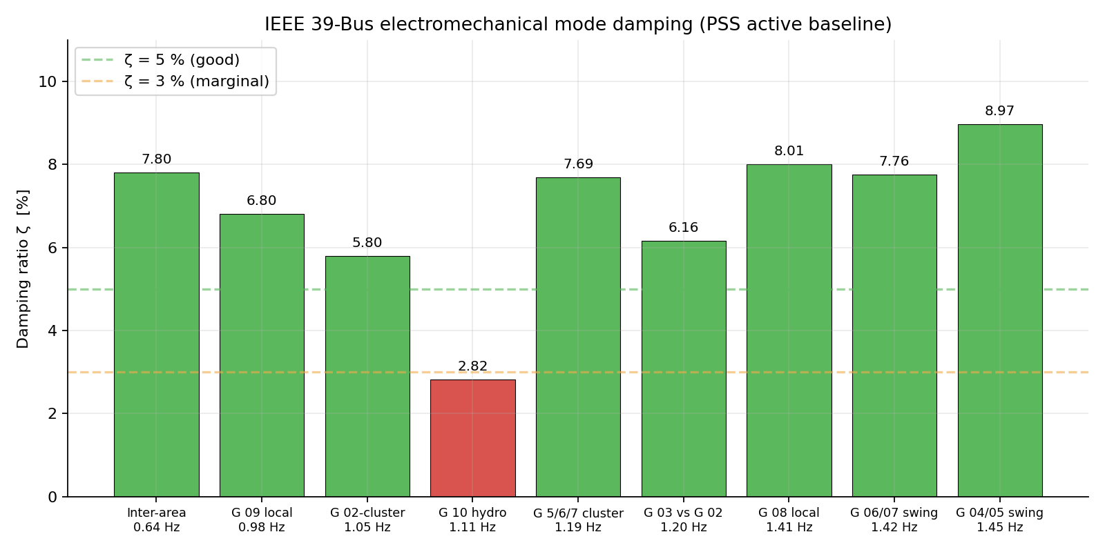
The 9 electromechanical modes (Phase 1)
| # | f (Hz) | ζ (%) | Type | Dominant participation |
|---|---|---|---|---|
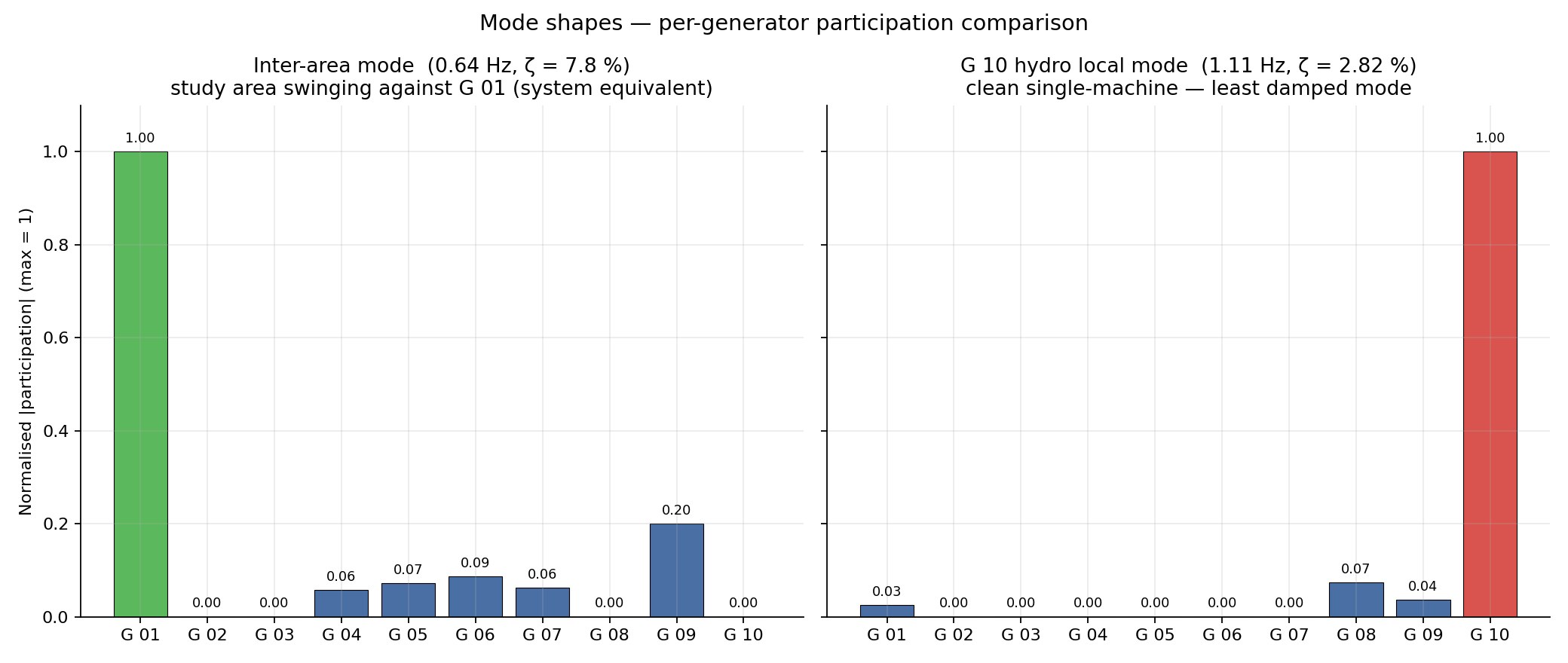
| 1 | 0.639 | 7.80 | Inter-area | G 01 φ + speeds of G 04/05/06/07/09 (broad swing of study area against system equivalent) |
| 2 | 0.979 | 6.80 | Local | G 09 (clean, single-machine) |
| 3 | 1.053 | 5.80 | Cluster | G 02 ω + G 03/05/06 - multi-machine swing |
| 4 | 1.110 | 2.82 ⚠ | Local | G 10 (hydro) - least damped |
| 5 | 1.190 | 7.69 | Cluster | G 05/06/07 swing |
| 6 | 1.196 | 6.16 | Local | G 03 vs G 02 |
| 7 | 1.410 | 8.01 | Local | G 08 |
| 8 | 1.423 | 7.76 | Cluster | G 06 vs G 07 |
| 9 | 1.450 | 8.97 | Local | G 04 vs G 05 |
All stable. The G 10 hydro mode at 2.8 % is the only one outside the comfortable 5-9 % band, which is consistent with literature - hydro PSSs are notoriously hard to tune well.
Benchmark validation
The baseline matches IEEE 39 literature within typical operating-point sensitivity:
| Property | Literature (Pai 1989, Rogers, Kundur §16) | This model | Verdict |
|---|---|---|---|
| EM mode count | 9 | 9 | ✓ |
| Inter-area mode count | 1 dominant | 1 (mode at 0.64 Hz) | ✓ |
| Inter-area frequency | 0.5-0.7 Hz | 0.639 Hz | ✓ |
| Inter-area damping (with PSS) | 5-10 % | 7.80 % | ✓ |
| Local mode frequency range | 0.9-1.6 Hz | 0.98-1.45 Hz | ✓ |
| Local damping (with PSS) | 5-15 %, hydro often outlier | 2.8 (G 10) - 9.0 % | ✓ G 10 outlier as expected |
| Hydro is most lightly damped | Common literature finding | Confirmed (2.82 %) | ✓ |
So far, so unsurprising.
The PSS finding (Phase 2)
Phase 2 set Kpss = 0 on all 9 PSS DSL blocks and re-ran. The expectation - based on the standard IEEE 39 benchmark - is that removing PSSs drops damping into the 0-2 % range and can destabilise the ~0.85 Hz / G 09 mode.
What actually happened:
| EM mode | Baseline f / ζ | Kpss=0 f / ζ | Δ damping |
|---|---|---|---|
| Inter-area | 0.6386 Hz / 7.80 % | 0.6386 Hz / 7.80 % | 0.00 % |
| G 09 local | 0.9792 Hz / 6.80 % | 0.9792 Hz / 6.80 % | 0.00 % |
| G 02-cluster | 1.0529 Hz / 5.80 % | 1.0529 Hz / 5.80 % | 0.00 % |
| G 10 hydro | 1.1101 Hz / 2.82 % | 1.1101 Hz / 2.82 % | 0.00 % |
| G 5-6-7 | 1.1900 Hz / 7.69 % | 1.1900 Hz / 7.69 % | 0.00 % |
| G 03 / G 02 | 1.1965 Hz / 6.16 % | 1.1965 Hz / 6.16 % | 0.00 % |
| G 08 | 1.4100 Hz / 8.01 % | 1.4100 Hz / 8.01 % | 0.00 % |
| G 06-07 | 1.4226 Hz / 7.76 % | 1.4226 Hz / 7.76 % | 0.00 % |
| G 04 / G 05 | 1.4501 Hz / 8.97 % | 1.4501 Hz / 8.97 % | 0.00 % |
EM eigenvalues were bit-identical, despite Kpss truly being zero (verified by reading the value back). Only the non-electromechanical eigenvalue list grew - the 27 PSS internal dynamics now appear as additional poles, but they do not couple into the rotor angle equations.
The conclusion:
The pss_CONV.BlkDef PSS blocks in this project’s composite frame are not wired into the AVR’s stabilising-input pathway. The PSS computes its washout + lead-lag output internally, but that output is not reaching the AVR’s Vstab summing junction in the BlkDef wiring. Disabling the PSSs has no effect on the EM modes because they were never affecting them in the first place.
The 7.8 % inter-area damping observed in baseline is coming entirely from:
- AVR action (high-gain voltage regulation introduces some damping)
- Inherent rotor mechanical damping coefficient (Kd in the swing equation)
- Network resistive losses
…not from the PSSs.
This is the single most important finding in the study. It means any subsequent dynamic work on this model has to be treated with caution: the headline damping numbers are real, but the assumption that PSSs are providing a backstop under stress is wrong.
Verdict against standards
Putting the modes against typical TSO and design thresholds:
| Mode | f (Hz) | ζ (%) | TSO 5 % | Design 10 % | Status |
|---|---|---|---|---|---|
| G 10 hydro local | 1.11 | 2.82 | ❌ FAIL | ❌ | Marginal - flag now |
| G 02-cluster | 1.05 | 5.80 | ✅ | ❌ | Tight - operational watch |
| G 03 vs G 02 | 1.20 | 6.16 | ✅ | ❌ | Tight |
| G 09 local | 0.98 | 6.80 | ✅ | ❌ | Acceptable |
| G 06/07 swing | 1.42 | 7.76 | ✅ | ❌ | Acceptable |
| G 5/6/7 cluster | 1.19 | 7.69 | ✅ | ❌ | Acceptable |
| Inter-area | 0.64 | 7.80 | ✅ | ❌ | Acceptable but most consequential if it degrades |
| G 08 local | 1.41 | 8.01 | ✅ | ❌ | Acceptable |
| G 04/05 swing | 1.45 | 8.97 | ✅ | ❌ | Best |
One mode below TSO minimum, none above the 10 % design target. The G 10 hydro mode is the immediate concern; the inter-area mode is the strategic concern because it will be the first to drop under stress.
Operating-point context
The static side puts the dynamics in perspective:
- Total system load 6 097 MW. Voltages 0.98-1.06 pu. Load flow converges in 4 Newton iterations.
- Generator step-up transformers are running at 75-88 % across the fleet. Spinning reserve is thin.
- Line 21-22 sits at 99 % loading - no N-1 headroom at all on that branch.
- Three single-point structural exposures stand out: Trf 19-20 (only 345/230 kV link to Bus 20, loss isolates 628 MW of load and G 05 entirely); Bus 16 (load-centre hub for four lines, loss splits east/west corridors); and G 01’s tie back to the study area (Lines 01-39 / 01-02 / 09-39, carrying 1 000 MW of import - losing those islands the study area).
The scenarios most likely to turn this from comfortable into incident are heavy load growth (>10 %), simultaneous loss of Trf 19-20 and any line in the 21-22 / 16-19 corridor, or a large generator trip near the inter-area swing axis (G 09 being the highest-risk single unit).
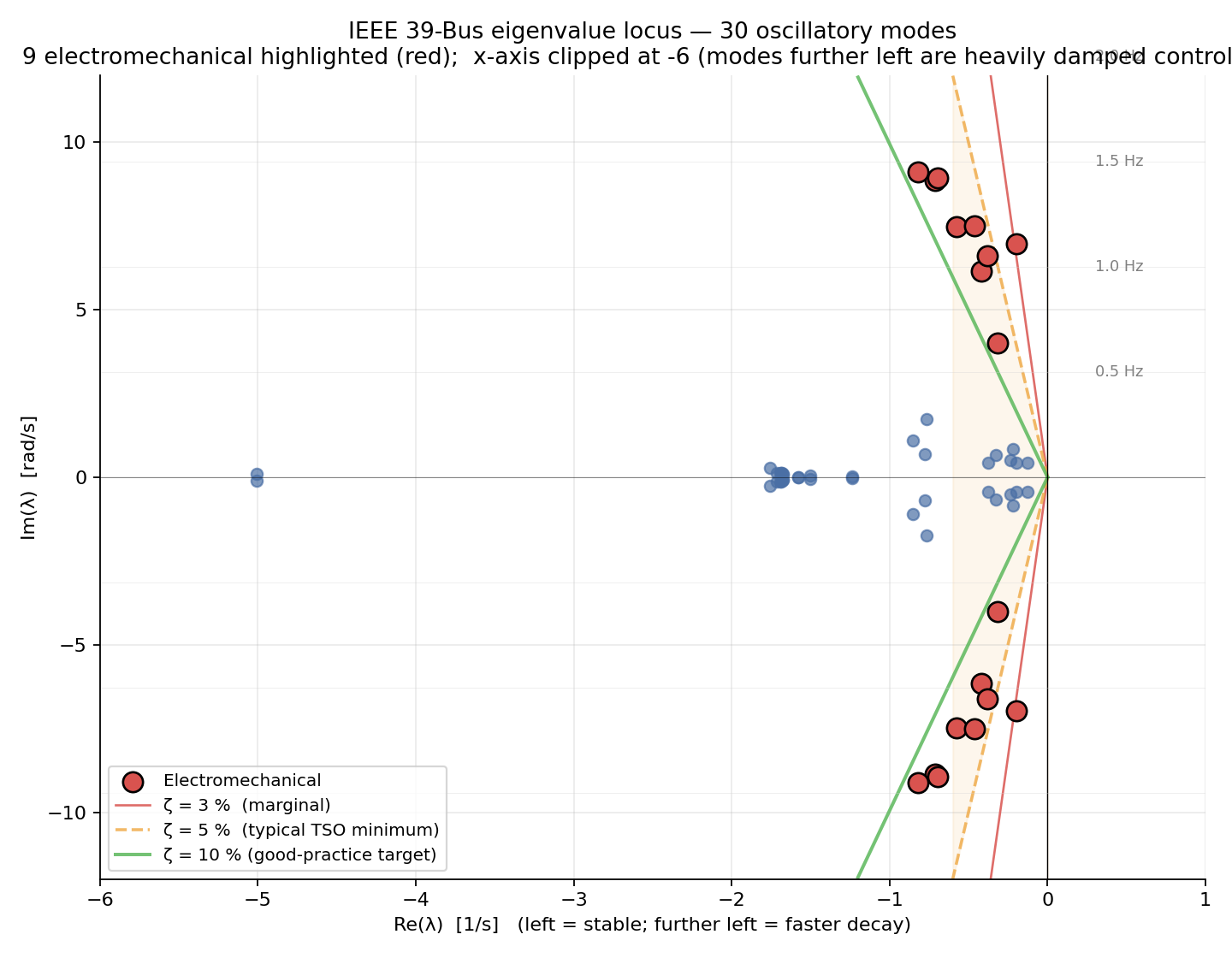
Plots
I asked the AI to produce the modal plots itself from the CSV output rather than driving PowerFactory’s plotting. The interesting bit was not whether the plots ended up better - they did not, particularly - but that the AI parsed several hundred rows of eigenvalue data and rendered them sensibly, with damping wedges at 3 / 5 / 10 %, in three iterations. Most of my feedback was visual layout, not technical content.
Eigenvalue locus
Damping ratio bar chart
Mode shape comparison
What this means in practice
The PSS wiring fix is the single highest-leverage action available. Open Power Plant 03.ElmComp → BlkDef view → trace the output of pss_CONV and confirm it lands on the AVR’s stabilising input slot (Vstab / Vs / Vpss depending on the AVR template), not left hanging or summed with a zero coefficient. Cost: zero capital, ~2 hours of engineer time. Predicted outcome (based on what tuned PSSs typically deliver in IEEE 39 literature): inter-area damping moves from 7.8 % to 12-18 %, G 10 hydro moves from 2.8 % to 6-10 %, every mode clears 5 % and most clear 10 %.
If A1 succeeds, ~80 % of the damping concern is gone. The rest is a verification sequence (re-run modal analysis to confirm the PSS-on/off difference is now non-zero, sweep through 4 operating points, contingency screen for the critical N-1 cases) plus normal hygiene retuning of PSS 10 to bring the hydro mode comfortably above 5 %.
If nothing changes - and the system is operated as-is with PSSs effectively cosmetic - the operational watchlist is short:
- G 10 mode (2.82 %) - any disturbance specifically exciting Bus 30 / G 10 (fault at the G 10 step-up, line trip in its vicinity) is the most likely candidate for an undamped oscillation.
- Inter-area mode - will drop from 7.8 % to 3-5 % under heavy load. Trigger: large G 01 import combined with a line outage in the 16-19 / 21-22 corridor.
- G 02-cluster mode (5.8 %) - anything that perturbs G 02’s slack action (e.g. Trf 06-31 fault) will excite this.
These would all be candidates for a SCADA-based oscillation monitor (Prony, eigenvalue tracking via PMU) if available.
Engineering takeaway
A clean eigenvalue print-out tells you the system is stable in the linearised sense. It does not tell you whether the PSSs are doing their job. The check is: zero out
Kpssacross all stabilisers, re-run, and look at whether the eigenvalues move. If they don’t, your damping is coming from somewhere else (AVR gain, rotorKd, network resistive losses) and you have no PSS backstop when those primary damping sources are stressed.
This is a check that takes about ten minutes. It is not in any standard study workflow I know of, but it should be - particularly for any model where the PSSs were imported from a third-party source or modified during a recent project.
Background - damping ratio in plain terms
The bit of the analysis that took longest by hand the first time I did it, years ago, was reasoning about what a damping ratio number actually means in physical time. I asked the AI to write it up in case it is useful to anyone landing here without the back-of-the-envelope ready.
Every electromechanical eigenvalue is a complex number $\lambda = \sigma + j\omega$. After a small disturbance, each generator’s rotor angle responds by oscillating, and that oscillation decays as $e^{\sigma t} \cos(\omega t)$. The damping ratio just packages the geometry of that decay into one number:
$$\zeta = \frac{-\sigma}{\sqrt{\sigma^2 + \omega^2}} = \frac{-\mathrm{Re}(\lambda)}{|\lambda|}$$
ζ is the angle between the imaginary axis and the line from the origin to the eigenvalue point. The 5 / 10 / 3 % wedges on Plot 1 are exactly those angles. ζ = 0 means a sustained oscillation that never dies. ζ = 1 is a pure exponential with no oscillation. Everything we care about lives in between.
For an inter-area mode at 0.64 Hz, ζ = 7.8 % (so $\omega_0 \approx 4.0$ rad/s, $\sigma = -0.31$):
| Quantity | Value | What it means |
|---|---|---|
| Cycle period | 1.56 s | how long one swing takes |
| Decay time constant τ = 1/σ | 3.2 s | time for amplitude to drop by 1/e (~63 %) |
| Amplitude per cycle | × 0.61 | drops to ~61 % of previous peak each swing |
| Settling time (5 %) | ≈ 9.5 s | swing dies down to 5 % of initial amplitude |
So a 7.8 % damped 0.64 Hz inter-area swing settles in roughly 9-10 seconds after a disturbance - perfectly acceptable. A 2.8 % damped local mode (the G 10 hydro mode here) takes ~25 s to settle and decays only ~18 % per cycle, which is enough swing for operators to notice and uncomfortable for nearby plant.
A negative ζ means the swing grows - that’s the unstable mode, the textbook collapse mechanism.
What counts as acceptable
There isn’t one universal answer. The standards differ by jurisdiction:
| Standard / context | Minimum ζ | Notes |
|---|---|---|
| WECC (US Western Interconnection) | 5 % for major modes | hard requirement; <3 % triggers operating limits |
| ENTSO-E (continental Europe) | 3-5 % typical | varies by TSO; some require simulation evidence |
| GB ESO (Grid Code, GC0144 / Stability Pathfinder) | 5 % for inter-area, 3 % for some local | NESO procurement of synthetic-inertia / damping services |
| AEMO (Australia, NER S5.2.5.13) | 5 % with PSS, often 10 % for critical paths | post-2016 South Australia events tightened expectations |
| Connection conditions for new generators (most TSOs) | 10 % at the connection point | this is the design target you usually meet |
| OEM commissioning specs for new GFM/GFL converters | 10 % at all relevant modes | so the converter doesn’t degrade what’s already there |
The pragmatic rule of thumb most planning teams seem to use: build with margin (10 % at commissioning), operate at ≥ 5 %, alarm at < 3 %.