MCP Toolcall and introspection

The basic concept of this exercise is to demonstrate how an MCP interface can provide a useful way of extracting and collecting data from an existing model. An engineer can of course open the model directly in whatever software package they are using, but this can be sometimes tedious and time consuming, especially when you are looking across a range of different equipment and parameters. Introspecting a project is useful as it lets you understand and query different parameters and settings and configurations, but really the key benefit of this is that you are creating a data pipeline between the software and the AI.

The results of the introspection don’t really tell us anyhthing we would not already know or be able to find out in other ways. The point of the exercise is the process and the results and accuracy of the retrieval.

IEEE 39-Bus Model

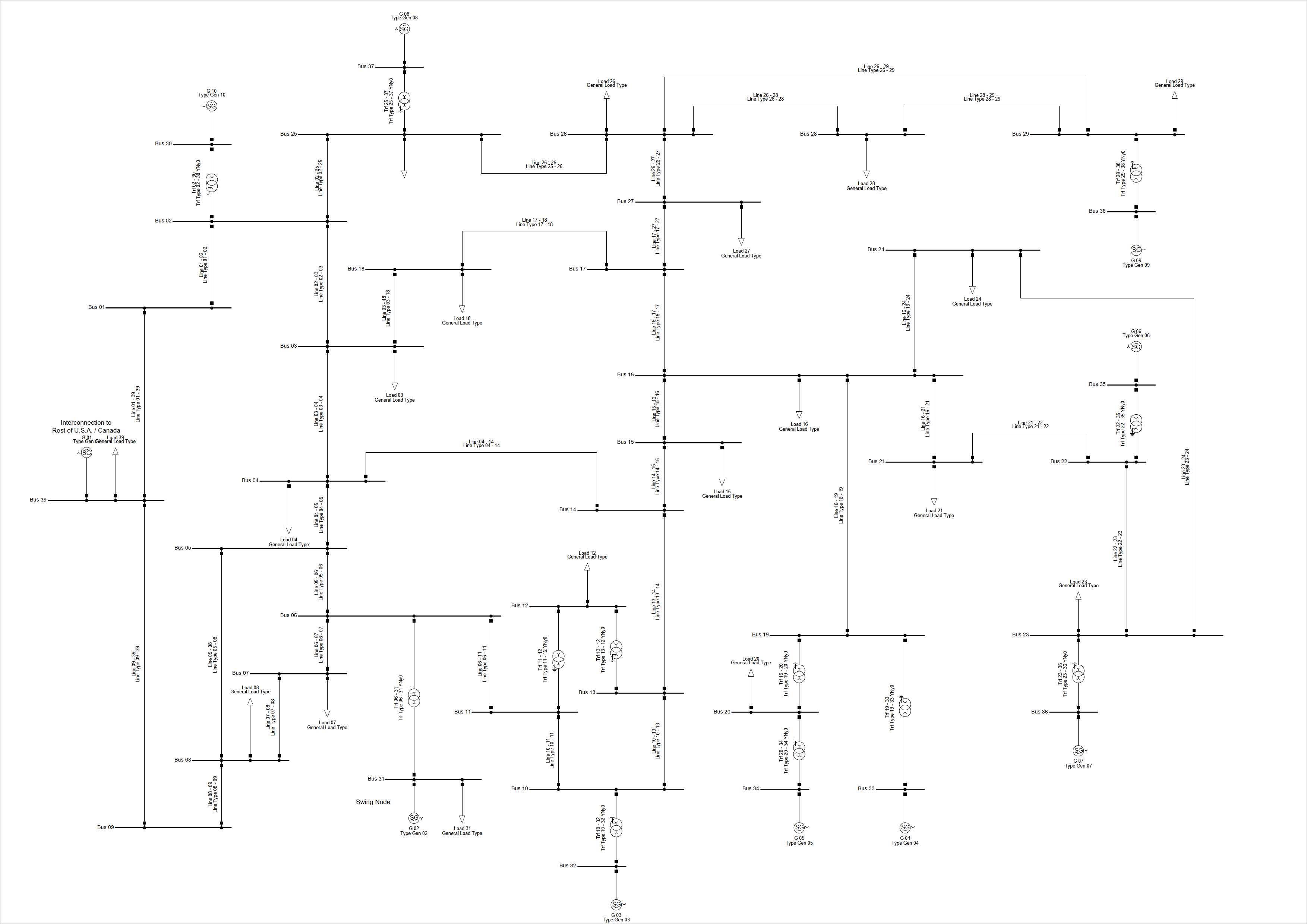
The IEEE 39-Bus model is a well known system (also called the New England system), and used a lot in academia and research. It is big enough to be interesting and complicated enough to show specific transmission level power systems analysis behaviour, but not so big that it gets unwieldy and difficult to follow. The network has a main transmission votlage of 345kV, and a number of strategic generators located through the system. Bus 39 and G39 represent the system external connection to a wider network.

IEEE 39-Bus Introspection

At a glance

Once the MCP server is loaded, I used a pre-defined set of rules and systems to carry out an ‘introspection’ of the plant. The idea, as noted above, is that the AI gets an overview of the system and can understand its structure and network topology, identify key generators, busbars loads and control systems.

Buses (ElmTerm)	39
Voltage levels	345 kV (28 buses, transmission) · 230 kV (1: Bus 20) · 138 kV (1: Bus 12) · 16.5 kV (10: gen terminals)
Lines (ElmLne)	34
Transformers (ElmTr2)	12
Synchronous machines (ElmSym)	10 (G 01–G 10)
DSL controllers	27 ElmDsl blocks across 10 ElmComp composite frames — i.e. one controller frame per generator
External grid (ElmXnet)	none (so no SCR calculable)
Operation scenario	none active
Total installed	14 535 MW / 17 100 MVA
Slack-equivalent	G 01 — 8 500 MW / 10 000 MVA (aggregates the NY–NE system, classic IEEE 39 convention)

(a) Generator dispatch & dynamic data

A1. Operating point (ElmSym)

Gen	Bus	P_dispatch (MW)	Q_setpt (MVAr)	cosφ	n_units	u_setp (pu)	Mode	Slack?
G 01	39	1 000	0	1.00	1	1.030	const-V	— (Pmax=8500)
G 02	31	0	0	1.00	1	0.982	const-V	✓ ip_ctrl=1
G 03	32	650	0	1.00	1	0.983	const-V	—
G 04	33	632	0	1.00	1	0.997	const-V	—
G 05	34	254	0	1.00	2	1.012	const-V	—
G 06	35	650	0	1.00	1	1.049	const-V	—
G 07	36	560	0	1.00	1	1.064	const-V	—
G 08	37	540	0	1.00	1	1.028	const-V	—
G 09	38	830	0	1.00	1	1.026	const-V	—
G 10	30	250	0	1.00	1	1.048	const-V	—

Notes:

• All in PV mode (av_mode = constv) — voltage-controlled. Q sets are 0 with cosφ=1 (LF will solve actual Q).
• G 02 is the swing bus (ip_ctrl=1). G 01 is not the slack despite its 8500 MW Pmax — its P is dispatched at 1000 MW and the rest is balanced by G 02. Classic IEEE 39 setup.
• G 05 has ngnum=2 — two parallel units of 300 MVA each (so Srated_total = 600 MVA, P_tot = 510 MW).

A2. Type data (TypSym) — all on the machine’s own MVA base

Type	Sgn (MVA)	Ugn (kV)	H (s)	xd	xq	x’d	x’q	x”d	T’d0 (s)	T”d0 (s)	iturbo
Gen 01	10 000	345	5.00	2.00	1.90	0.60	0.80	0.40	2.10	0.033	1 (round)
Gen 02	700	16.5	4.33	2.07	1.97	0.49	1.19	0.35	1.55	0.036	1
Gen 03	800	16.5	4.48	2.00	1.90	0.42	0.70	0.36	1.21	0.042	1
Gen 04	800	16.5	3.58	2.10	2.06	0.35	1.33	0.28	0.95	0.040	1
Gen 05	300	16.5	4.33	2.01	1.86	0.40	0.50	0.27	1.06	0.034	1
Gen 06	800	16.5	4.35	2.03	1.93	0.40	0.65	0.32	1.44	0.040	1
Gen 07	700	16.5	3.77	2.07	2.04	0.34	1.30	0.31	0.94	0.045	1
Gen 08	700	16.5	3.47	2.03	1.96	0.40	0.64	0.32	1.32	0.039	1
Gen 09	1 000	16.5	3.45	2.11	2.05	0.57	0.59	0.45	1.30	0.039	1
Gen 10	1 000	16.5	4.20	1.00	0.69	0.31	0.50	0.25	3.16	0.040	0 (salient)

Three things stand out:

1. G 01 is the system equivalent — connected directly at 345 kV (no step-up, no Trf 01-xx exists), Sgn 10 GVA, H = 5 s, modelling the rest of the NY-NE interconnection.
2. G 10 is the only hydro unit — iturbo = 0, much lower xd (1.0 vs ~2.0), large saliency, very long T’d0 (3.16 s).
3. All others are round-rotor thermal with classical reactances (xd ≈ 2.0, xdss = xqss = 0.27–0.45). Equal d/q subtransients is the standard simplification.

System inertia: weighted-by-MVA mean H ≈ 4.4 s at machine base, ≈ 4.4 GW·s/GVA × 17.1 GVA = 75 GW·s total stored kinetic energy. Removing G 01 (which is the equivalent rest-of-system, not a real machine) leaves ≈ 30 GW·s for the 9 study-area machines.

---

(b) Controller architecture

B1. Composite frame inventory

10 ElmComp frames, 27 ElmDsl total. Pattern:

Composite	Slots / DSL blocks	Generator
Power Plant 02	AVR 02, GOV 02, PSS 02	G 02
Power Plant 03	AVR 03, GOV 03, PSS 03	G 03
Power Plant 04	AVR 04, GOV 04, PSS 04	G 04
Power Plant 05	AVR 05, GOV 05, PSS 05	G 05
Power Plant 06	AVR 06, GOV 06, PSS 06	G 06
Power Plant 07	AVR 07, GOV 07, PSS 07	G 07
Power Plant 08	AVR 08, GOV 08, PSS 08	G 08
Power Plant 09	AVR 09, GOV 09, PSS 09	G 09
Power Plant 10	AVR 10, GOV 10, PSS 10	G 10
Rest of U.S.A. / Canada	(empty — 0 DSL)	G 01

Confirmed: 9 plants × 3 slots = 27 ElmDsl, matching the project introspect count.

Architectural takeaway: every machine except G 01 has the classic AVR + GOV + PSS triplet. G 01, being the system equivalent, is run as an uncontrolled inertia + impedance representation — appropriate for studies where the dynamics of NY-NE are out of scope.

B2. Sample DSL parameters — Power Plant 03

Block	Parameters returned
AVR 03	Tr = 0.0 (regulator input filter time constant — instantaneous)
GOV 03	Pmax = 1.0, Pmin = 0.0, T1 = 0.2 s, T2 = 1.0 s, T3 = 0.6 s, T4 = 0.6 s
PSS 03	T1 = 3.0 s, T2 = 0.2 s, T3 = 2.0 s, T4 = 0.2 s, Vmax = +0.2 pu, Vmin = −0.2 pu

Caveats:

• The DSL tool only surfaces the parameter names it knows about (WECC + common IEEE legacy names). The AVR returning just Tr strongly suggests it’s a minimal IEEE-DC1A or simplified Type-1 with most other parameters under non-standard names — they’re in the model but the tool didn’t enumerate them. Same for GOV.
• The PSS pattern (two lead-lag stages T1/T2 + T3/T4 + a ±0.2 pu output limiter) is the classic IEEE PSS1A / IEEEST single-input stabilizer signature.
• The GOV signature (Pmax/Pmin + T1–T4) is consistent with a TGOV1 / IEEEG1 simplified thermal governor.

If you want a definitive identification of the DSL block models, the next step is to read each block’s typ_id (BlkDef reference) — that gives the actual block-frame name. Tell me and I’ll fetch those.

---

(c) Network topology

C1. Voltage levels in use

kV	Buses	Role
345	28 (Bus 01–29 minus 12, 20 + Bus 39)	transmission backbone
230	1 (Bus 20)	sub-transmission island fed from Bus 19
138	1 (Bus 12)	sub-transmission island fed from Bus 11 & 13
16.5	10 (Bus 30–38 + … wait, Bus 30 not 39)	generator terminals (G 02–G 10)

Note: G 01 sits at Bus 39 (345 kV) directly — no step-up.

C2. Lines (TypLne) — all 34 are 345 kV

Sampled 6 of 34. Identical pattern across all sampled types: uline = 345 kV, xline = 0.30 Ω/km, sline = 1.0 kA (rated current). Variation is purely in R and B:

Line type	rline (Ω/km)	xline (Ω/km)	bline (μS/km)	sline (kA)
Line Type 01 - 02	0.0255	0.300	3.60	1.0
Line Type 03 - 04	0.0183	0.300	2.20	1.0
Line Type 09 - 39	0.0120	0.300	10.16	1.0
Line Type 16 - 17	0.0236	0.300	3.19	1.0
Line Type 17 - 27	0.0225	0.300	3.94	1.0
Line Type 26 - 28	0.0272	0.300	3.49	1.0

frnom = 60 Hz (US system, as expected for IEEE 39).

The uniform xline = 0.3 Ω/km and uniform 1 kA rating are typical of benchmark-system simplifications — the author tuned R and B per branch to hit the canonical IEEE 39 impedances while keeping X identical and ratings unconstrained. No 230 kV or 138 kV lines exist — those buses are reached only through transformers.

C3. Transformers (TypTr2) — all 12, all YNy0 vector group

Transformer	Sn (MVA)	HV (kV)	LV (kV)	uk (%)	Pcu (kW)
Trf Type 02 - 30 (G 10)	1 000	345	16.5	18.10	0
Trf Type 06 - 31 (G 02)	700	345	16.5	17.50	0
Trf Type 10 - 32 (G 03)	800	345	16.5	16.00	0
Trf Type 11 - 12	300	345	138	13.06	1 440
Trf Type 13 - 12	300	345	138	13.06	1 440
Trf Type 19 - 20	1 000	345	230	13.82	7 000
Trf Type 19 - 33 (G 04)	800	345	16.5	11.37	4 480
Trf Type 20 - 34 (G 05)	300	230	16.5	10.81	1 620
Trf Type 22 - 35 (G 06)	800	345	16.5	11.44	0
Trf Type 23 - 36 (G 07)	700	345	16.5	19.04	2 450
Trf Type 25 - 37 (G 08)	700	345	16.5	16.25	2 940
Trf Type 29 - 38 (G 09)	1 000	345	16.5	15.62	8 000