Using AI to Introspect an EPRI PSCAD Grid Forming Inverter Model
The team at Manitoba (PSCAD) and Deepak Ramasubramanian from EPRI have produced a publicly available Grid Forming Inverter model in PSCAD format. This is a really useful resource, as GFM technology is still very much in the early days and despite a lot of papers on the subject there is very little standardisation on how they actually work and what they can and cannot do. In this case study I use the AI to probe and carry out a series of sweeps on the PSCAD model to see what it can do, what its strengths are and any gaps.
I have found generally that most engineers, get the general principle of a GFM easily enough, but don’t really have enough experience of them to contextualise what their behaviour means in real world output of fault level, voltage regulation and synthetic inertia.
Grid Forming Inverter Models | PSCAD
Problem
Part of the problem with GFM technology is that they are fairly complicated designs, and the control systems are not always clear or well established. When working in a PSCAD environment - and as powerful as PSCAD is, let’s be honest - its user interface for signals and control system modelling is a little bit clumsy. This makes reviewing someone else’s model of a control system difficult and time consuming, as it is not always obvious how the control is set up, and it can be difficult to follow and trace signals through.
EPRI GFM Model
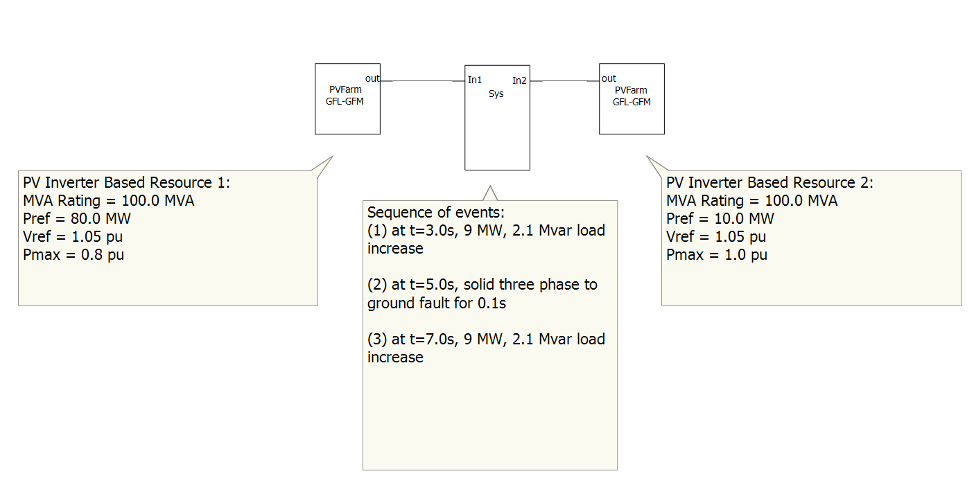
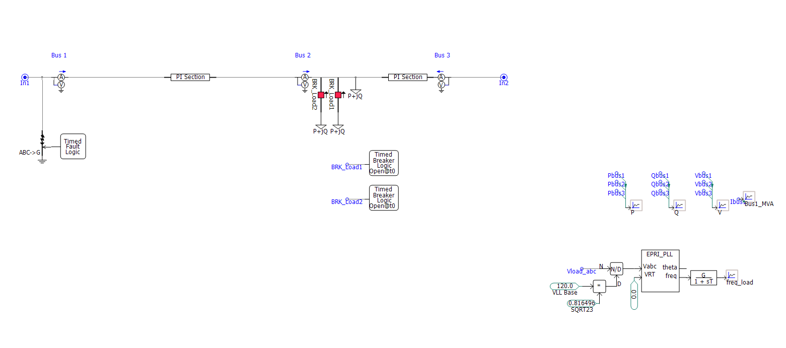
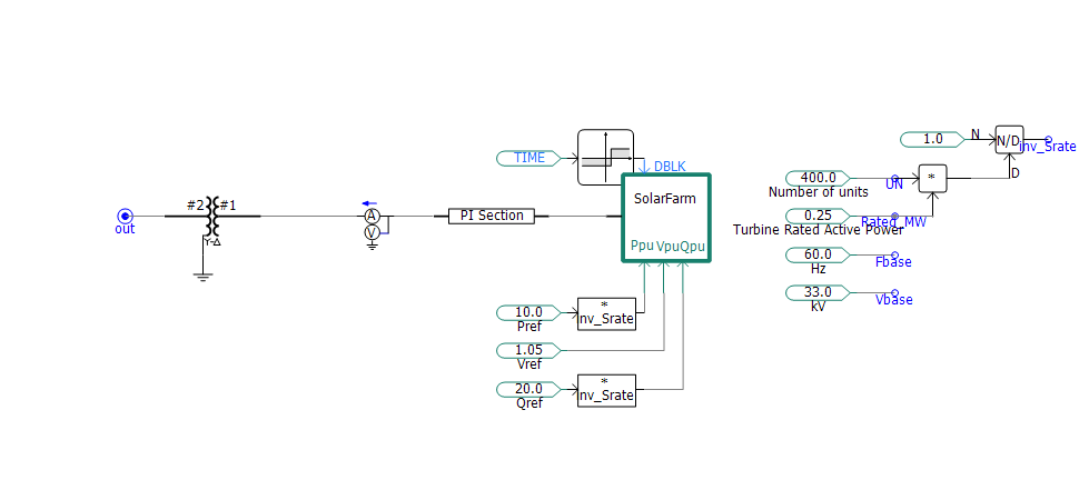
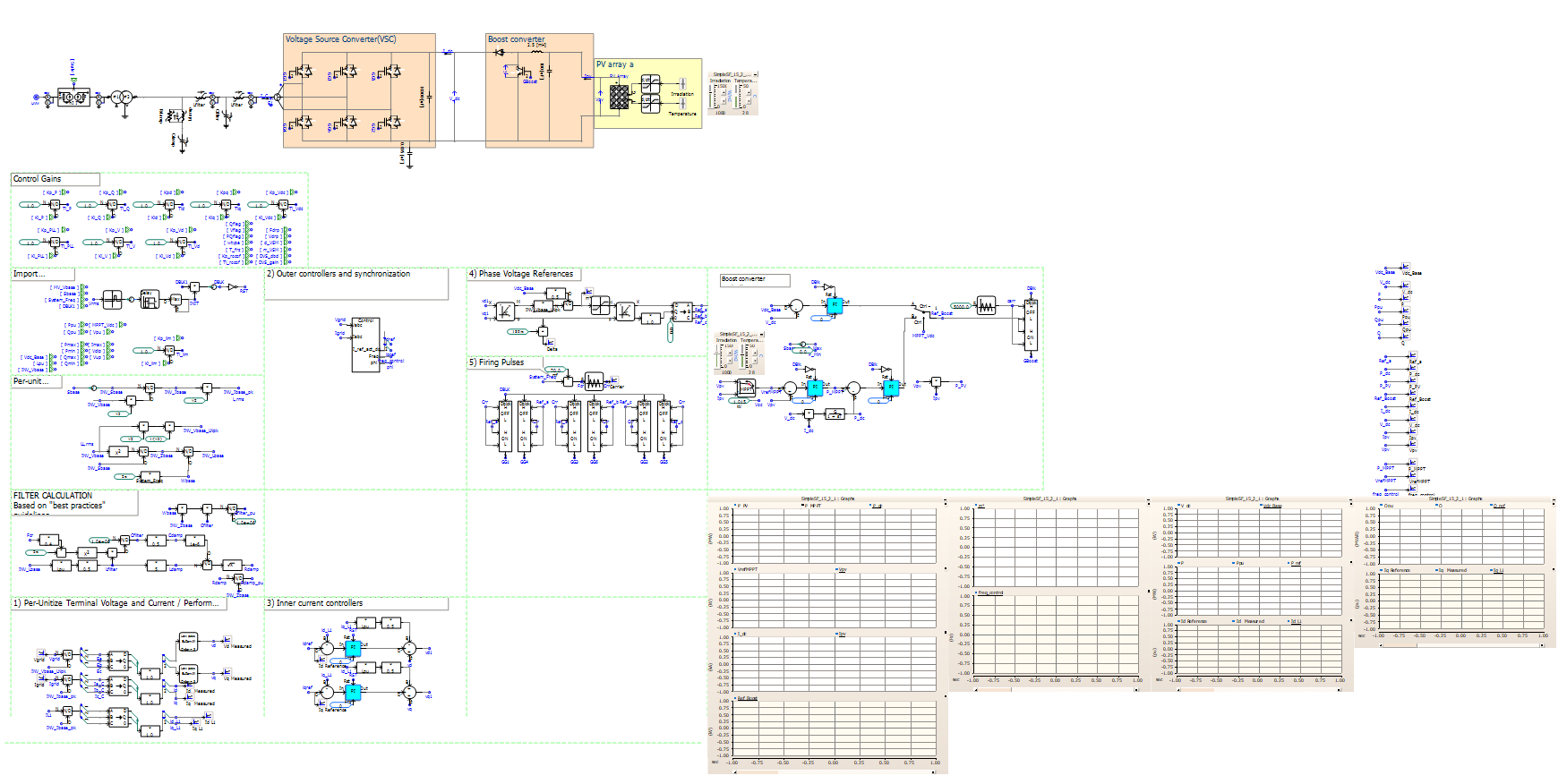
The EPRI GFM model is actually based on two GFM Solar farms, connected into a single equivalent system (Fig 1), that has a number of loads connected in the central section, with a few breaker control timers to apply faults and load events (Fig 2). The solar sites are both identical and have a simple transformer and cable PI section (Fig 3) and then a detailed implementation of the PV system that shows the GFM control (Fig 4). The first three figures are easy enough to follow, but figure 4 is where you need a strong coffee and a bit of time to trace things through by hand.
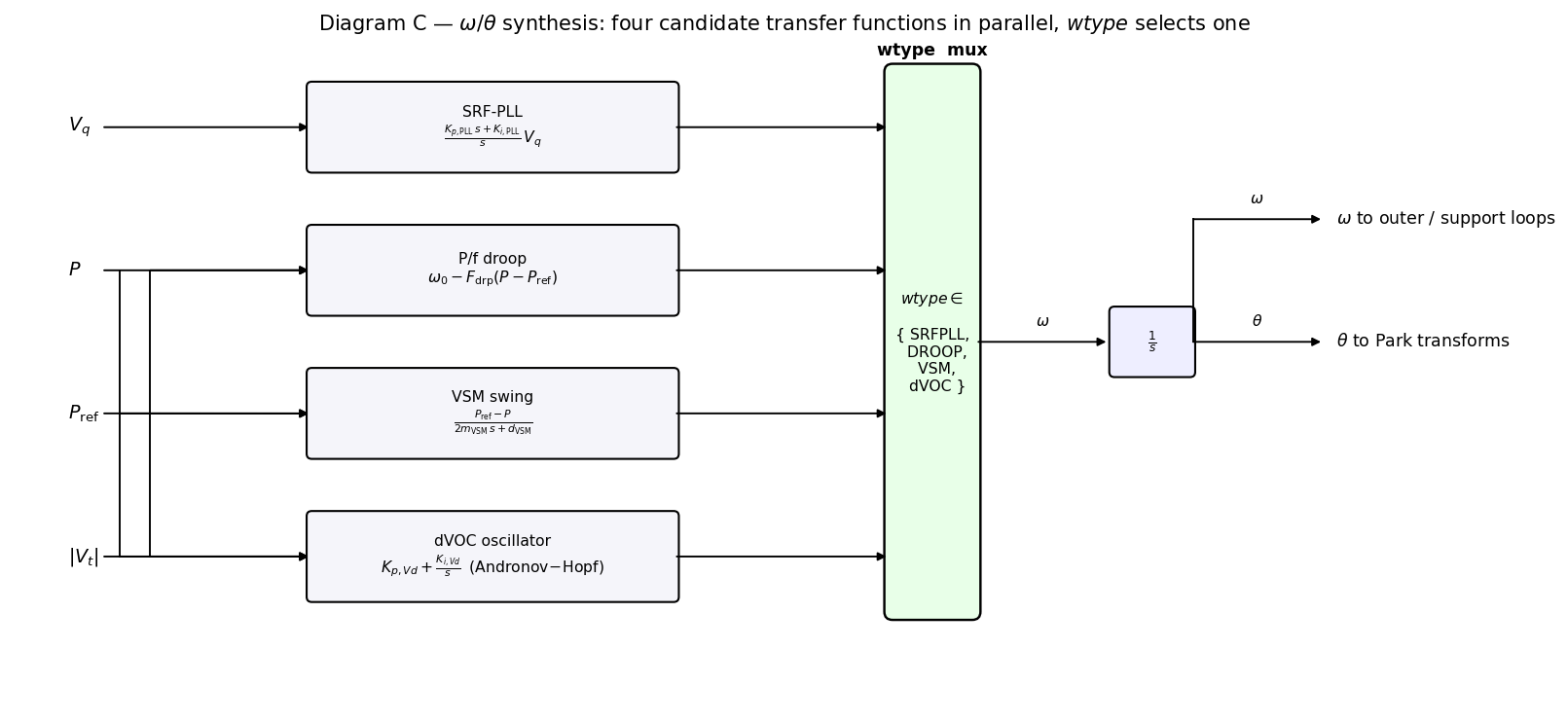
The EPRI generic GFM is a single controller (SimpleSF) that creates its own voltage-source behaviour using one of four user-selectable angle-and-frequency methods. The selector is the wtype parameter; the rest of the controller (P/Q outer loops, V outer loop, dq inner current loop, current limiter, FRT freeze logic) stays the same across all four. In addition to the four main modes (shown in the table below), there are a number of other settings of interest:
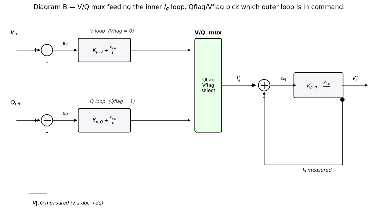
Qflag-1puts the reactive controller in voltage-regulating mode,0in Q-regulating mode.Vflag-0selects the fast-terminal-voltage path,1a slower Q→V regulator.PQflag-"Q"gives Q priority in the current-magnitude limiter,"P"gives P priority.
In the as-shipped model these are Qflag=1, Vflag=0, PQflag="Q" for all four wtype choices, so the mode regression is a clean apples-to-apples comparison of the angle-synthesis method only.
Mode (wtype) |
How frequency / angle is synthesised | Key gain set | Character in this scenario |
|---|---|---|---|
SRFPLL - PLL-GFM |
Synchronous-Reference-Frame PLL tracks the terminal voltage; the inverter still uses a PLL but a fast inner V loop makes its terminals look stiff. | Kp_PLL=20, Ki_PLL=200, Kp_V=0.5, Ki_V=100 |
Cleanest start-up (~0.3 s settle), lowest fault-current peak (4.94 kA on PV1) - the PLL re-locks within a fraction of a cycle so the limiter engages early. |
DROOP |
Direct P/f and Q/V droop - frequency is set by f = f₀ − Fdrp · (P − Pref). No PLL in the angle loop. |
Fdrp=30, Vdrp=22.22 |
Slower start-up (0.7 s ringing, PV2 P-overshoots to 60 MW). Larger first-cycle fault current (6.08 kA) because there’s no PLL to fast-track angle. |
VSM - Virtual Synchronous Machine |
Swing equation: 2H · dω/dt = Pref − P − D·(ω − ω₀). Should give synthetic inertia. |
m_VSM=0.01 (inertia coefficient), d_VSM=0.3 (damping) |
Indistinguishable from Droop in the as-shipped configuration. With m=0.01 the swing equation degenerates to steady-state droop. To see the inertia character, m_VSM would need to be lifted to 0.1–1.0 and d_VSM retuned. |
DVOC - Dispatchable Virtual Oscillator |
A nonlinear oscillator (Andronov-Hopf) whose limit cycle is the desired voltage; ω/V emerge as oscillator states. | Kp_Vd=3, Ki_Vd=10 |
Fastest settle (~0.4 s), smallest start-up overshoot, closest to nominal frequency in steady state (the integrator pulls f toward 60 Hz between events). Mid-range fault current (5.35 kA). |
Method
The starting point of the analysis was the assumption that the GFM model is correct and does what we expect. This is pretty much a given as it was produced by EPRI and PSCAD, so errors in the model are unlikely but possible so we should never be complacent. When tackling a project like this, the best approach is to be slow and methodological to make sure that you understand the key parts and don’t go down too many rabbit holes. The key steps completed were:
- Introspected the model top-down - confirmed it’s the EPRI generic positive-sequence GFM packaged by Manitoba Hydro: two 100 MVA aggregated PV farms back-to-back, separated by a 3-bus 120 kV system with no synchronous generation, sized 400 × 0.25 MW units = 100 MW per farm.
- Mapped the controller architecture -
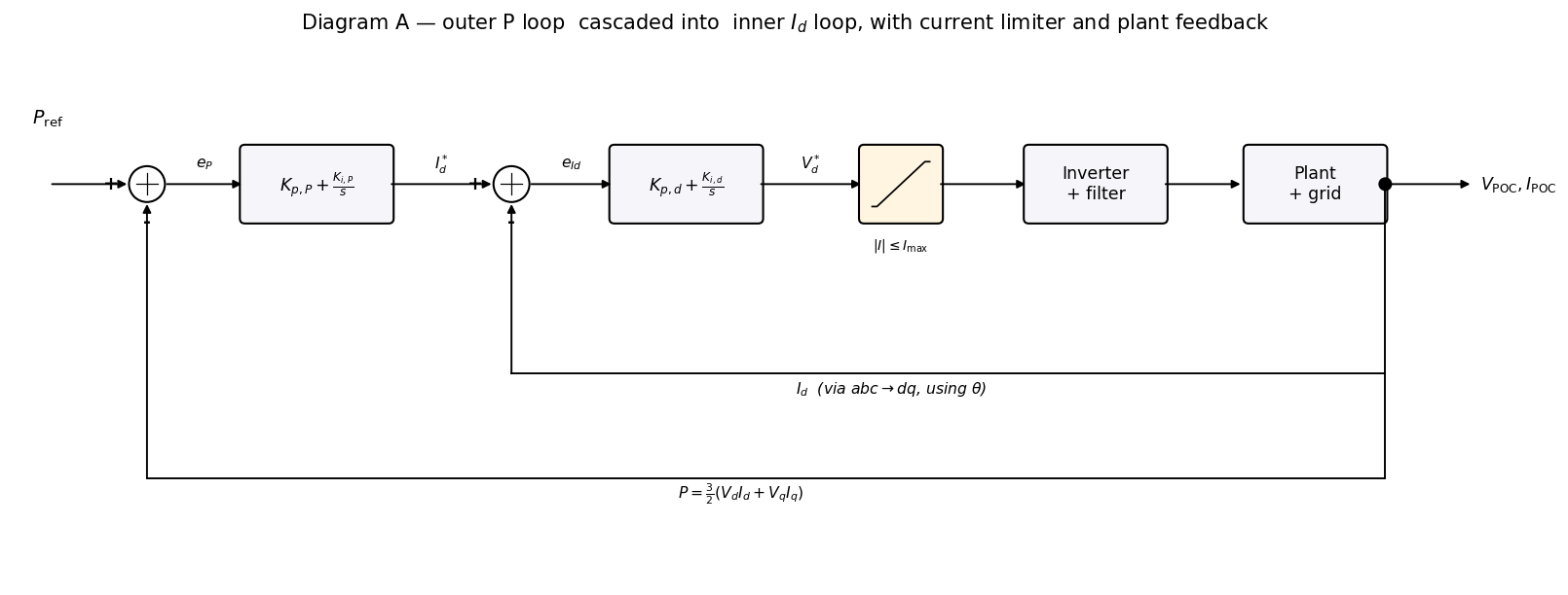
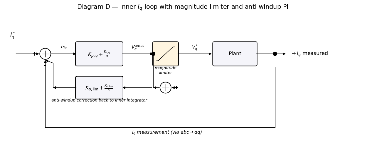
SimpleSFcore, decomposed into PLL, P/Q outer loops, V loop, dq inner current loop, current-limiter with anti-windup, FRT freeze logic. Same controller, four selectable angle-synthesis modes (PLL/Droop/VSM/dVOC) chosen by thewtypeflag. - Developed a 5-stage test plan with an approval header and human input.
- Executed 9 simulation runs, each 10 s of EMT at 5 µs, ~5 min wall clock, ~120 MB of
.outdata per run, 115 measured channels per run. - Generated about 100 plots (one signal per pane, per your preference), then 5 cross-stage synthesis figures.
Introspecting the control systems
With a GFM, the key bit is understanding the control systems and control loops of the various systems in place and how they work. As a first step I got the AI to run through the systems it could see and then use matplotlib to create a simplified series of control function diagrams based on what it could see
The test plan
As noted above, the key thing with running and understanding any system is to develop a test plan. In this case, I had a bit of backwards and forwards to develop a plan with Claude, we eventually settled on the following:
| Stage | What it tests | Variation from baseline |
|---|---|---|
| 1.1 Baseline | Does the as-shipped model ride through the canonical scenario? | None - as-shipped: PLL-GFM, PV1 Pmax=0.8, PV2 Pmax=1.0 |
| 3.A Droop 3.B VSM 3.C dVOC |
Mode regression - does each advertised GFM mode pass the same FRT test? | wtype switched on both farms, gains otherwise unchanged |
| 2.1 50 ms (2.2 = baseline 100 ms) 2.2 200 ms 2.3 300 ms |
Fault-duration sensitivity - is there a critical clearing time? | Fault DF swept; mode held at PLL |
| 4 Asymmetric Pmax | What happens when one farm is capacity-limited? | PV1 Pmax reduced 0.8 → 0.5 |
| 5 Single-phase A-G | Boundary test - does the positive-sequence model handle unbalance? | Fault phases B and C disabled, only A-G |
Synthetic inertia - how it’s handled in this model
In a synchronous-machine grid, the rotor’s spinning mass resists changes in frequency. That’s pure Newtonian physics:
$$2H \frac{d\omega}{dt} = P_\mathrm{mech} - P_\mathrm{elec} \qquad H = \frac{1}{2} \frac{J \omega_s^2}{S_\mathrm{base}}$$
The constant H (units: seconds) tells us how many seconds of rated power the rotor’s kinetic energy could supply if you stopped the prime mover. Real synchronous machines: H = 2–6 s. The bigger H is, the slower the frequency changes for a given power imbalance. That’s what we mean when we say a grid “has inertia.”
In an inverter-only system there is no rotor and no kinetic energy. The DC link is sized for power flow, not for inertial buffering. Frequency can change as fast as the controller permits - and for a fast PLL-based GFL inverter, that’s very fast. Hence the problem. The EPRI generic GFM has all three plumbed in:
| Mechanism | What it does | Where it lives in this model |
|---|---|---|
| Virtual Synchronous Machine (VSM) | Solves the swing equation in software: 2m·dω/dt = Pref − P − d·(ω−ω₀) and uses the resulting ω as the frequency reference |
wtype = VSM mode; gains m_VSM (inertia coefficient) and d_VSM (damping) |
| Frequency droop with finite bandwidth | When the outer P loop has a finite time constant, the inverter resists rapid power changes in a way that looks like inertia for a few hundred ms | wtype = DROOP mode; gain Fdrp = 30 |
| ROCOF support | Measures df/dt directly and adds Kp_rocof · df/dt to the active-power command |
Available via Kp_rocof parameter (currently 0, i.e. disabled) |
Results - what we found
About the model
The EPRI generic GFM is robust. In every test we ran - four GFM modes, four fault durations from 50 ms to 300 ms, asymmetric Pmax, single-phase fault - every simulation completed cleanly, no trips, no chatter, full recovery. The model is FRT-capable in every mode it advertises.
The different operating modes have different fingerprints but converge to the same operating point. PLL-GFM is fastest and quietest. dVOC has the best steady-state frequency tracking. Droop and VSM are essentially identical at the as-shipped m_VSM=0.01 (the inertia is too small to matter - to see VSM character you need m ≈ 0.1–1.0). Mode choice affects dynamics - settling time, overshoot, fault current peak - not where the system ultimately sits.
This might sound underwhelming, but it is exactly what we expected to find, the detail is in the dynamics and understanding what and how it does things:
What’s the same across all four
- Same outer P, Q, V loops. Mode flag changes only how the angle/frequency reference is generated. Power-sharing between PV1 and PV2 is determined by
PmaxandVref, not bywtype. - Same FRT machinery -
Imax=1.2pu current limit,Vdip=0.8/Vup=1.3ride-through window,T_frz=0.2 spost-fault state-freeze. - Same DC-link control -
Kp_Vdc=1,Ki_Vdc=20, MPPT enabled. - All four ride through the 100 ms 3-φ-G fault with no trips and full recovery.
What changes between modes
- Settling time and ringing during start-up and load steps - ranges from 0.3 s (PLL) to 0.7 s (Droop/VSM).
- First-cycle fault-current peak - PLL is best (4.94 kA), Droop/VSM are worst (~6 kA), dVOC sits in the middle (5.35 kA).
- Steady-state frequency error - dVOC closes it best (59.96 Hz vs 59.95 Hz for the others; small but consistent).
- Frequency-trace fingerprint during a fault - different in shape, all clean in outcome.
About faults and fault duration
No critical clearing time within 300 ms. The peak fault current is set by the first half-cycle subtransient before the limiter engages, so it’s identical at 50/100/200/300 ms (4.94 kA on PV1). To actually find CCT you’d have to push past 1 s where the DC-link energy budget becomes binding. For any realistic protection coordination this is a non-issue.
The model handles A-G unbalance numerically, despite EPRI’s “unvalidated” disclaimer. It doesn’t trip, doesn’t oscillate, recovers cleanly. That’s not the same as saying it’s accurate against a vendor reference - but on this network it is at least stable.
Synthetic inertia response
Almost no synthetic inertia. Two reasons:
m_VSM = 0.01in VSM mode. To put that in synchronous-machine units, you’d want H ≈ 2–6 s for a real-machine equivalent. m_VSM=0.01 gives an effective H around an order of magnitude below that. The swing equation degenerates to a steady-state droop relationship - which is exactly why Stage 3 showed VSM and Droop modes were indistinguishable. The “VSM” badge is checked on the box, the inertia value is set near zero.Kp_rocof = 0(ROCOF support disabled). The signal path is wired but the gain is zero, so no df/dt-based active power injection is occurring.
So when the disturbances hit, the system has:
- Electrical droop through the outer P loop (yes -
Fdrp=30works in all four modes) - No synthetic inertia worth measuring
To get an island that behaves electromechanically like a synchronous-machine grid, you’d need to:
- Set
wtype = VSMand liftm_VSMto 0.1–1.0, then re-tuned_VSM(probably 1–3) so it’s underdamped just enough to give visible inertial swing without ringing. This is the proper GFM approach. - Optionally additionally enable
Kp_rocof(start ~0.05, tune up). This adds an explicit ROCOF-based active-power injection on top of whatever the outer loop is doing - a “fast frequency response” channel. - Make sure the DC link can supply the inertial energy. Synthetic inertia is a real exchange - when the inverter pushes extra power for a few hundred ms during a frequency dip, that energy has to come from somewhere. For a PV inverter with no battery and MPPT enabled, there’s no inertial reserve; the inverter would have to curtail steady-state output to keep headroom. This is the system limitation that defines how much synthetic inertia you can actually deliver. A BESS or curtailed PV with
Pref < Pmppis the usual answer.
What it all means
For the model itself: the EPRI generic GFM in PSCAD is fit for purpose as a positive-sequence-domain demonstrator. Use it for FRT studies, control-mode comparison, and dispatch-architecture exploration. Don’t use it for unbalanced-fault certification or DC-side disturbance studies - those are outside its validated envelope.
For grid design: in a 100% IBR island, frequency control is a system property, not a controller property. Any combination of capacity-asymmetric GFMs without AGC will land at a steady-state frequency dictated by their droop settings and the load. If you want 60.00 Hz you need either (a) a frequency reference machine (synchronous gen, big BESS in PLL-grid-following mode following an external clock), or (b) a secondary control layer doing AGC. The choice of GFM mode does not by itself solve this - though dVOC pulls closer to nominal than the others through its integrator action.
Mode choice affects dynamics, not steady-state outcomes. All four GFM modes ride through every disturbance and converge to the same operating point. What actually shifts the operating frequency of an islanded 100 % IBR system is not the GFM mode - it’s whether you have AGC, secondary control, or a frequency reference. Stage 4 proved this: with PV1 capacity-limited and no AGC, frequency settles at 58.98 Hz post-event regardless of how clever the inverter’s angle synthesis is. The grid-design lesson dominates the controller-design lesson.
For the control-mode debate: the four-mode taxonomy in the EPRI document is more a difference of fingerprint than of capability. All four ride through the same fault, settle to the same operating point, and hand off the same load increments to the headroom inverter. Mode choice matters for transient quality, not for steady-state outcomes. So vendors arguing “GFM mode X is uniquely capable” should be challenged to produce a scenario where the settled behaviour differs - in this model, none does.
Engineering takeaway
This was a really good bit of AI blended exploratory learning. PSCAD models of complicated systems are hard work to navigate through and doing it manually is time consuming and often tedious, unless the originator has been very diligent with notes and documentation. Using the AI we managed to introspect the model pretty thoroughly, understand what its control structure was, how it was configured, and what were the key parameters. Then we were able to develop a test plan, run through a number of simulations and prove that the model behaved as expected. The AI summary that it got very excited about, but would be obvious to most senior engineers was the lack of active power control in the system.