AVR model build - from PDF datasheet to a tested PSCAD model with AI

The Idea - AVR transfer function diagram

Modelling control systems in PSCAD is generally not too difficult, but it can be frustrating and time consuming, as the PSCAD libraries are not extensive. As a simple experiment I decided to test out the new MCP interface I had built, and use an AI to build an implementation of a synchronous machine AVR. AVR models are generally given in a PDF form showing a series of transfer functions for the AVR, usually aligning with one of the standard IEEE models. The datasheet also contains all the standard settings for the specific instance of the machine settings such as gain values, time constants and limits.

Using the MCP interface I had already developed, I was able to get the AI to build the implementation relatively easily and cleanly within PSCAD and follow the process step-by step, using the layout already created. The interesting part is that although the AVR is complicated, the transfer functions are all ‘simple’ maths, and I was able to define a simple test plan with the AI, and get it to test its response with a series of test step responses, to identify any broken links.

Where the AI struggled was building a sub-module to containerise the created AVR module. I pretty much had to hand walk it through that process. This was partly because the PSCAD documentation on this process is not exactly clear.

What the AI actually did

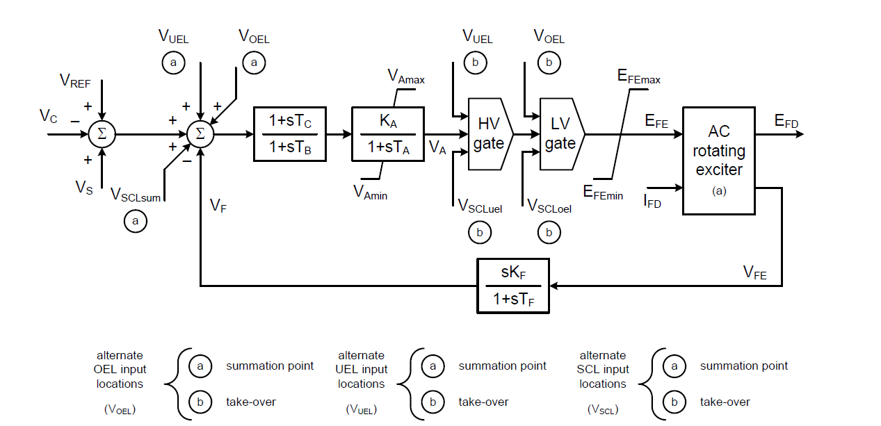
The model I decided to build and test, was a relatively simple AC1C exciter, as shown in the IEEE 421.5 standard. This is a simple exciter with enough detail in to be interesting but not so much it gets confusing. The associated incoming OEL, UEL, SCL functions are flexible enough to be either summation of takeover type.

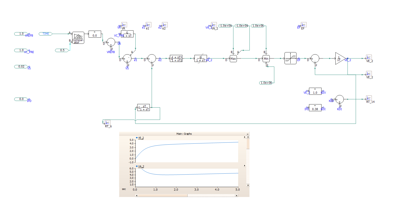
The output result from PSCAD can be seen below. All the key elements are there and correctly wired up. Although on the first pass it made a mess of the HV and LV gates and included some direct invisible connection (wireless label) for the feedback loops that I could not find easily - this was not wrong, but it makes auditing hard. Even with several attempts at iteration for the layout, it was still less than ideal.

Working through an MCP-style direct interface to PSCAD, it was possible to show that a fully integrated workflow is possible with an AI agentic approach. The human intervention was primarily on sanity checking and helping to ensure the layout was graphically consistent. The key achievements were:

1. Read the AVR datasheet and transfer functions PDF and extracted the block diagram structure, parameters and limits.
2. Built the model in PSCAD block-by-block, wiring up summing junctions, gains, lead-lag stages and limiters.
3. Designed a test plan - small-signal steps on the reference, large-signal step, limiter exercise - to prove the model behaved as specified.
4. Ran the tests, captured the responses, and compared them against the expected behaviour from the datasheet.
5. Spotted where the response did not match, identified the likely cause, and refined the model.

The Test Plan and Results

ID	What it does	What we look for	Result
T01	VREF +5 % step at t=0.5 s	EFD rises monotonically, VA stays below ±VAmax, EFE eventually clamps at +6.03 (rectifier ceiling). Shape, not just final value.	EFD smooth ramp 0 → 6.0 over ~10 s; VA peaks ≈9; EFE saturates at 6.03 from t≈7 s. Stabiliser visible in err2 dip.
T02	VREF +20 % step	VA hits +14.5 (VAmax) and stays there; EFE clamped at +6.03 immediately after step	Both limits bind; EFD reaches 6.03 in ~2 s.
T03	VREF −10 % step	Symmetric negative response; VA reaches −14.5 (VAmin); EFE reaches −5.43 (EFEmin)	All lower limits bind correctly.
T04	LV-gate take-over: c_lvtake = +2.0 while VA is saturating positive	EFE clamped at exactly +2.0; EFD settles at 2.0	LV gate min(VA, V_LVTAKE) = 2.0 confirmed.
T05	HV-gate take-over: c_hvtake = +1.0 while VA goes deeply negative	EFE forced to +1.0; EFD steady at 1.0	HV gate max(VA, V_HVTAKE) = 1.0 confirmed.
T07	IFD demagnetisation (IFD = 1.0, no VREF step)	VFE biased by KD·IFD = 0.38 at t=0; integrator drives VE negative; regulator gradually compensates	Visible negative excursion of EFD then slow recovery.
T08	VS injection (+0.02, no VREF step)	err1 = +0.02 throughout; EFD rises positive (verifies VS additive sign)	VS-only response identical in shape to a 2 % VREF step.

What went well and less well

As with all ideas, there is a lot of time spent helping the AI / MCP interface understand what is going on and how to carry out the actions, this was expected and a well trodden path for MCP interfaces, or jumping to odd conclusions, where it chained together 6 summation ports for no real reason. The headaches were primarily that the PSCAD library were missing a couple of the transfer functions I wanted, and we had to navigate a workaround using equivalent summation transfer functions. This was a key step forward in model building, but in reality I could have built it faster myself and with a lot less hassle.

Layout, this is where AI and humans diverge pretty sharply. When building a model by hand I usually spend a lot of time, laying out the wires and nodes (spaghetti) carefully so I can follow it and debug it. The AI approach is a lot more haphazard, and looks messy in a way that ‘upsets’ me, even when given lots of rules for layout, and overlapping signals and wires. Conceptually, this makes sense as an AI sees data paths and data flows, it does not really think visually, and getting it to structure and order graphical layouts nicely is surprisingly hard and time consuming.

On reflection, the really interesting bit was not “the AI built a model.” The interesting bit was that the AI designed and ran the validation test plan itself, recognised when the response was wrong, and iterated. That is the agentic loop in practice - not a single tool call, but plan → act → check → refine, with the engineer reviewing at each step. It was also more thorough than I would have been if doing it myself, i would have done a couple of spot checks, eyeballed it and moved on. It did however miss the obvious tests, of checking if it initialised cleanly without any wobble, and a series of smaller events inside the normally operating range to make sure it was working as expected, and not just focusing on the clamp behaviour.

What we learnt

The main learning outcome of this is that with a suitable MCP interface and a bit of time building and helping the AI understand how to interface with PSCAD and carry out the tasks, this sets the framework for significant future time saving. The agentic process and self-testing and diagnoses was very strong and turned this from a simple tool call into something very interesting.