Using PSCAD with Pandapower to initialise complex networks

Technical Note TN-006
For more detail, figures and results - download the PDF
Download PDFPSCAD Loadflow initialisation
One of the common headaches on large PSCAD models is how to initialise the network for specific loadflow cases. This usually needs a second model to be created in DIgSILENT or PSS/E and then used to calculate the various machine angles and terminal voltages. This can be a frustrating process. This example shows how pandapower can be coupled with PSCAD to resolve this headache.
Using an MCP server, it is possible for the AI to create a simplified 1-to-1 model of the PSCAD network in pandapower and solve any loadflow scenario using an established Newton-Raphson iteration model. Once the network is solved, the AI can then pass the settings to PSCAD through the MCP layer.
1. PSCAD and Loadflow
PSCAD is a very powerful software package, but it is fundamentally a time-domain solution program, designed to solve differential equations of complex items of plant for a given set of specific values (the initial parameters). However, it does not have any specific loadflow analysis tools. That means an engineer has to manually set all the machine and voltage source terminal voltages and angles in order to get the required power flow solution for MW and MVAr.
There are obviously various ways of doing this, and traditionally, depending on the complexity of the network, it has been a combination of running a series of simulations in a conventional analysis package such as DIgSILENT or PSS/E and noting the various source initial values, and then copying them into the PSCAD model. This usually is a frustrating process that takes some trial and error. More recently PSCAD has also introduced a tool called PRSIM which allows these results to be mapped across.
The problem in both cases is the time and effort taken to work the values out, and then the potential drift between the two models can start to become a real headache. What may seem like small differences such as transformer tap settings and correct modelling of cable shunt capacitances can start to add up on complex networks.
2. Pandapower
Pandapower is a simple(?!) open source python based loadflow and short circuit analysis tool for modelling networks. It includes representations of all main power systems components, but does not include any detailed control systems.
It is particularly interesting for use with AI and PSCAD for a number of reasons. Firstly, it is all python code and AI - are getting really good at coding now. This means that getting the AI to create the model is pretty much trivial. Second, provided that an appropriate MCP interface and skill sets are defined the AI can build the model directly from the PSCAD model and keep it in sync at all times. This means that there is much less risk of model drift, and when discrepancies do occur the AI can see both models simultaneously and bug-hunt to find the cause of the problem.
3. Testing on an IEEE 39-Bus Model
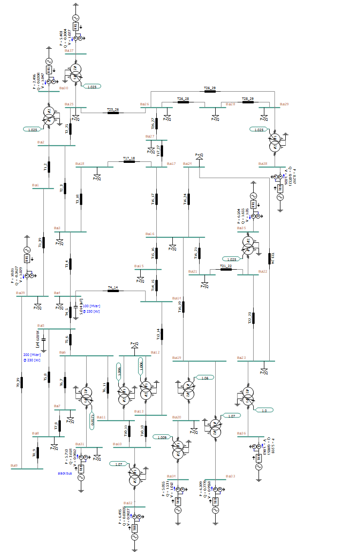
The IEEE 39-Bus model is a well known industry benchmark, and has been set up by MHI already in PSCAD, as can be seen below. The standard PSCAD model includes all the generators as simple voltage sources rather than as synchronous machines - as that would get a bit challenging - but the same principle applies with the source terminal voltage and angles.
In order to test the concept, I got the AI to setup 4 test cases in Pandapower with different loading scenarios, and then check the correlation between the two models. A simple base case scenario (S1) and then two load variations keeping the network balance the same (S2 and S3) and then finally a case with generation shifted away from the East to the North East.
| Case | Definition | Load MW | Gen MW | Losses MW | Vmin / Vmax pu |
|---|---|---|---|---|---|
| S1 Base | Model’s own dispatch, 100% load. Sanity check that pandapower reproduces the PSCAD file’s existing init values. | 6150 | 6178 | 28.9 | 0.982 / 1.075 |
| S2 Light | All loads scaled to 60% (P and Q), all generator P scaled to 60%. | 3690 | 3702 | 11.8 | 0.982 / 1.106 |
| S3 Peak | All loads scaled to 110%, all generator P scaled to 110%. | 6764 | 6799 | 34.9 | 0.982 / 1.066 |
| S4 Dispatch shift | 100% load, 450 MW moved from the east to the north-east. G6 and G7 back off, G8 and G9 pick up. | 6150 | 6195 | 45.3 | 0.982 / 1.074 |
The overall correlation was pretty tight, and whilst some differences were present they were not significant. The total network differences between the PSCAD and pandapower models were fairly modest, with (as expected) the slack bus picking up the MW difference and the MVAr differences being spread through the network. The detailed results are in the Appendix below. The following observations are made:
-
There was a small systematic bias identified in every case. The EMT P and Q are higher at all ten machines, every terminal voltage is a fraction lower, and angles lead by 0.01–0.035°.
-
EMT generates 10–18 MW / 31–40 MVAr more than pandapower, scaling with load. G1 (slack) takes the P mismatch; dQ spreads across the PV machines, G3 largest.
-
This is thought to be representation difference (line charging, transformer model, or fixed-P sources not holding their Pinit) rather than an initialisation error.
4. Summary
This small project is something that started off as a bit of fun, but has rapidly become a key use case and a great time saver when working on real problems and scenarios. The dual configured PSCAD-Pandapower model lets me run both models simultaneously and configure the PSCAD model for pretty much any case I want without having to do a lot of manual labour and iteration. There is the added bonus that as pandapower is native python there was no need to build another MCP server or set up any tools or skillsets for it.
As a small ‘fun’ experiment I might get the AI to see if it can replace all the voltage sources with a sub-module of a synchronous machine, and then rewire and test again!
Download Technical Note 006 - Coupling PSCAD and Pandapower (PDF)
Appendix - Detailed Results
S1 Base - model dispatch, 100% load
| Gen | Bus | P pp MW | P emt MW | dP MW | Q pp MVAr | Q emt MVAr | dQ MVAr | V pp pu | V emt pu | dV pu | ang pp deg | ang emt deg | dang deg |
|---|---|---|---|---|---|---|---|---|---|---|---|---|---|
| G1 | 39 | 987.1 | 990.6 | +3.5 | -38.5 | -35.8 | +2.7 | 1.0300 | 1.0296 | -0.0004 | -10.06 | -10.06 | +0.000 |
| G2 | 31 | 571.3 | 572.8 | +1.5 | 361.7 | 365.8 | +4.1 | 0.9820 | 0.9814 | -0.0006 | -1.38 | -1.36 | +0.024 |
| G3 | 32 | 650.0 | 650.9 | +0.9 | -1.7 | 3.3 | +5.0 | 0.9831 | 0.9824 | -0.0007 | 2.01 | 2.04 | +0.030 |
| G4 | 33 | 632.0 | 633.3 | +1.3 | 77.2 | 81.2 | +4.1 | 0.9972 | 0.9966 | -0.0006 | 3.20 | 3.22 | +0.025 |
| G5 | 34 | 508.0 | 509.5 | +1.5 | 148.8 | 152.5 | +3.8 | 1.0123 | 1.0118 | -0.0005 | 1.86 | 1.88 | +0.024 |
| G6 | 35 | 650.0 | 651.4 | +1.4 | 157.9 | 161.9 | +4.0 | 1.0493 | 1.0488 | -0.0005 | 5.05 | 5.08 | +0.026 |
| G7 | 36 | 560.0 | 560.9 | +0.9 | 79.1 | 82.6 | +3.5 | 1.0635 | 1.0631 | -0.0004 | 7.75 | 7.78 | +0.031 |
| G8 | 37 | 540.0 | 541.1 | +1.1 | -31.5 | -28.2 | +3.3 | 1.0278 | 1.0275 | -0.0003 | 2.25 | 2.28 | +0.028 |
| G9 | 38 | 830.0 | 832.3 | +2.3 | 5.3 | 8.7 | +3.4 | 1.0265 | 1.0260 | -0.0005 | 7.57 | 7.58 | +0.014 |
| G10 | 30 | 250.0 | 251.9 | +1.9 | 75.7 | 79.3 | +3.6 | 1.0475 | 1.0471 | -0.0004 | -3.50 | -3.48 | +0.023 |
| Total | 6178.4 | 6194.7 | +16.3 | 833.9 | 871.4 | +37.4 |
S2 Light - 60% load, gens 60%
| Gen | Bus | P pp MW | P emt MW | dP MW | Q pp MVAr | Q emt MVAr | dQ MVAr | V pp pu | V emt pu | dV pu | ang pp deg | ang emt deg | dang deg |
|---|---|---|---|---|---|---|---|---|---|---|---|---|---|
| G1 | 39 | 586.7 | 588.7 | +2.0 | -226.7 | -224.8 | +1.9 | 1.0300 | 1.0299 | -0.0001 | -10.06 | -10.06 | +0.000 |
| G2 | 31 | 342.8 | 343.7 | +0.9 | 204.4 | 207.9 | +3.5 | 0.9820 | 0.9816 | -0.0004 | -5.06 | -5.05 | +0.014 |
| G3 | 32 | 390.0 | 390.6 | +0.6 | -148.2 | -143.9 | +4.3 | 0.9831 | 0.9826 | -0.0005 | -3.06 | -3.04 | +0.018 |
| G4 | 33 | 379.2 | 380.0 | +0.8 | -30.6 | -27.1 | +3.5 | 0.9972 | 0.9968 | -0.0004 | -2.26 | -2.24 | +0.015 |
| G5 | 34 | 304.8 | 305.7 | +0.9 | 67.4 | 70.6 | +3.3 | 1.0123 | 1.0119 | -0.0004 | -3.04 | -3.03 | +0.015 |
| G6 | 35 | 390.0 | 390.9 | +0.9 | 20.8 | 24.1 | +3.3 | 1.0493 | 1.0490 | -0.0003 | -1.23 | -1.22 | +0.015 |
| G7 | 36 | 336.0 | 336.6 | +0.6 | -17.0 | -14.0 | +2.9 | 1.0635 | 1.0633 | -0.0002 | 0.35 | 0.37 | +0.018 |
| G8 | 37 | 324.0 | 324.7 | +0.7 | -101.7 | -99.0 | +2.7 | 1.0278 | 1.0276 | -0.0002 | -2.75 | -2.73 | +0.016 |
| G9 | 38 | 498.0 | 499.5 | +1.5 | -119.4 | -116.9 | +2.6 | 1.0265 | 1.0263 | -0.0002 | 0.32 | 0.33 | +0.006 |
| G10 | 30 | 150.0 | 151.1 | +1.1 | -14.4 | -11.5 | +3.0 | 1.0475 | 1.0472 | -0.0003 | -6.20 | -6.18 | +0.014 |
| Total | 3701.5 | 3711.4 | +9.9 | -365.5 | -334.4 | +31.1 |
S3 Peak - 110% load, gens 110%
| Gen | Bus | P pp MW | P emt MW | dP MW | Q pp MVAr | Q emt MVAr | dQ MVAr | V pp pu | V emt pu | dV pu | ang pp deg | ang emt deg | dang deg |
|---|---|---|---|---|---|---|---|---|---|---|---|---|---|
| G1 | 39 | 1088.9 | 1092.9 | +3.9 | 11.9 | 14.8 | +2.9 | 1.0300 | 1.0295 | -0.0005 | -10.06 | -10.06 | +0.000 |
| G2 | 31 | 628.4 | 630.1 | +1.6 | 408.4 | 412.7 | +4.4 | 0.9820 | 0.9813 | -0.0007 | -0.44 | -0.41 | +0.028 |
| G3 | 32 | 715.0 | 715.9 | +0.9 | 42.7 | 48.0 | +5.3 | 0.9831 | 0.9823 | -0.0008 | 3.32 | 3.35 | +0.034 |
| G4 | 33 | 695.2 | 696.6 | +1.4 | 110.5 | 114.8 | +4.3 | 0.9972 | 0.9966 | -0.0006 | 4.59 | 4.62 | +0.029 |
| G5 | 34 | 558.8 | 560.5 | +1.7 | 173.3 | 177.2 | +4.0 | 1.0123 | 1.0118 | -0.0005 | 3.11 | 3.13 | +0.027 |
| G6 | 35 | 715.0 | 716.5 | +1.5 | 200.5 | 204.7 | +4.2 | 1.0493 | 1.0487 | -0.0006 | 6.68 | 6.71 | +0.030 |
| G7 | 36 | 616.0 | 617.0 | +1.0 | 109.2 | 113.0 | +3.7 | 1.0635 | 1.0631 | -0.0004 | 9.67 | 9.71 | +0.035 |
| G8 | 37 | 594.0 | 595.2 | +1.2 | -9.2 | -5.7 | +3.5 | 1.0278 | 1.0274 | -0.0004 | 3.51 | 3.54 | +0.032 |
| G9 | 38 | 913.0 | 915.5 | +2.5 | 45.1 | 48.7 | +3.7 | 1.0265 | 1.0260 | -0.0005 | 9.44 | 9.45 | +0.017 |
| G10 | 30 | 275.0 | 277.1 | +2.1 | 102.3 | 106.1 | +3.8 | 1.0475 | 1.0470 | -0.0005 | -2.83 | -2.80 | +0.026 |
| Total | 6799.4 | 6817.4 | +18.0 | 1194.6 | 1234.3 | +39.7 |
S4 Dispatch shift - G6/G7 -450 MW, G8/G9 +450 MW
| Gen | Bus | P pp MW | P emt MW | dP MW | Q pp MVAr | Q emt MVAr | dQ MVAr | V pp pu | V emt pu | dV pu | ang pp deg | ang emt deg | dang deg |
|---|---|---|---|---|---|---|---|---|---|---|---|---|---|
| G1 | 39 | 1003.5 | 1007.0 | +3.4 | -22.3 | -19.5 | +2.8 | 1.0300 | 1.0296 | -0.0004 | -10.06 | -10.06 | +0.000 |
| G2 | 31 | 571.3 | 572.7 | +1.4 | 366.2 | 370.3 | +4.1 | 0.9820 | 0.9814 | -0.0006 | -2.71 | -2.69 | +0.024 |
| G3 | 32 | 650.0 | 650.8 | +0.8 | 2.5 | 7.5 | +5.0 | 0.9831 | 0.9824 | -0.0007 | 0.47 | 0.50 | +0.030 |
| G4 | 33 | 632.0 | 633.3 | +1.3 | 77.7 | 81.7 | +4.0 | 0.9972 | 0.9966 | -0.0006 | -0.26 | -0.24 | +0.025 |
| G5 | 34 | 508.0 | 509.5 | +1.5 | 149.0 | 152.7 | +3.8 | 1.0123 | 1.0118 | -0.0005 | -1.61 | -1.58 | +0.024 |
| G6 | 35 | 400.0 | 401.7 | +1.7 | 118.0 | 121.9 | +3.9 | 1.0493 | 1.0488 | -0.0005 | -4.14 | -4.12 | +0.023 |
| G7 | 36 | 360.0 | 361.2 | +1.2 | 42.6 | 46.0 | +3.4 | 1.0635 | 1.0632 | -0.0003 | -2.44 | -2.41 | +0.028 |
| G8 | 37 | 740.0 | 740.6 | +0.6 | -2.7 | 0.6 | +3.4 | 1.0278 | 1.0274 | -0.0004 | 6.71 | 6.74 | +0.031 |
| G9 | 38 | 1080.0 | 1082.4 | +2.4 | 101.0 | 104.6 | +3.6 | 1.0265 | 1.0259 | -0.0006 | 16.08 | 16.09 | +0.010 |
| G10 | 30 | 250.0 | 251.8 | +1.8 | 121.4 | 125.0 | +3.6 | 1.0475 | 1.0471 | -0.0004 | -2.67 | -2.65 | +0.024 |
| Total | 6194.8 | 6211.2 | +16.4 | 953.4 | 991.0 | +37.5 |